Model-based learning for high-dimensional wireless systems

---

Baptiste CHATELIER

Supervisors: Luc LE MAGOAROU, Matthieu CRUSSIERE, Vincent CORLAY

PhD defense - INSA Rennes - January 30, 2026

General context

CONTEXT

• Funded by Mitsubishi Electric R&D Centre Europe (Rennes)

• Hosted at IETR laboratory, INSA Rennes (Rennes)

• Partially hosted at the Institute of Research and Technology b<>com (Rennes)

COLLABORATIONS

• Aalto University, Finland

• Chalmers University of Technology, Sweden

  • Research stay at Chalmers between September-December 2024

Scientific context

MODEL-BASED MACHINE LEARNING: MOTIVATIONS

Typical data processing setting:

• We observe a large number of correlated variables, explained by a small number of independent factors.

G. Peyré, “Manifold models for signals and images”, in Computer Vision and Image Understanding, 2009

M. Elad, “Sparse and Redundant Representations: From Theory to Applications in Signal and Image Processing”, Springer, 2010

Nir Shlezinger, Yonina C. Eldar, “Model-Based Deep Learning”, Foundations and Trends in Signal Processing, 2023

There are two complementary approaches to handle this situation:

• Signal processing
  • Model-based
  • Large bias
  • Low complexity

• AI / ML
  • Data-based
  • Low bias
  • High complexity

Hybrid approach \(\rightarrow\) model-based machine learning

Use models to structure, initialize or optimize learning methods

• Make models more flexible: reduce bias of signal processing methods
• Guide machine learning methods: reduce their complexity

Thesis problematic

Can MB-ML be used to get interpretable and low-complexity solutions in wireless communications?

OUR WORK

• Investigate the MB-ML framework for wireless communication problems

Research axes

(A1) Location-to-channel mapping

(A2) Hardware impairments

(A3) Channel compression

RESEARCH AXIS 1 Location-to-channel mapping

Chapters 4 and 5 of the manuscript

LOCATION-TO-CHANNEL MAPPING

• Propagation channel coefficients are needed in many communication problems

• Radio digital twin \(+\) ray-tracing tools \(\rightarrow\) \(\mcD = \left\{ \bx_i, \bH\left(\bx_i\right) \right\}_{i=1}^N\)

J. Hoydis et al., “Sionna: An Open-Source Library for Next-Generation Physical Layer Research”, 2022

Drawbacks:

• Long generation time (\(\sim\) hours for large scenes)

• Database size proportional to the number of locations (\(\sim\) Gb for large scenes)

Problem 3.1: MB-ML for radio-environment compression

\[ \mini{\ftheta}{\espo{\norm{\textcolor{#B22222}{\ftheta\left(\bx\right)}-\bH\left(\bx\right)}{\mathsf{F}}^2}{\left(\bx, \bH \left(\bx\right)\right) \sim p_{\bx,\bH}}}{\ftheta \in \mathcal{H}} \]

where:

\[ \begin{aligned} \textcolor{#B22222}{\ftheta} \colon \mbbR^3 &\longrightarrow \mbbC^{N_a \times N_s} \\ \bx &\longrightarrow \hat{\bH}\left(\bx\right) \end{aligned} \]

• Goal: find \(\textcolor{#B22222}{\ftheta}\)

• Error measure: reconstruction error (\(\ell_{\mathsf{F}}\) norm)

ML APPROACH: INR

• Use of the Implicit Neural Representation concept:

  • Neural networks are universal function approximators
  • Using \(\bx\) one can design and train \(\ftheta\) in a supervised manner to learn a representation of \(\bH\left(\bx\right)\)

K. Hornik, M. Stinchcombe, and H. White, “Multilayer feedforward networks are universal approximators”, in Neural Networks, 1989

G. Cybenko, “Approximation by superpositions of a sigmoidal function”, in Mathematics of Controls, Signals and Systems, 1989

N. Rahaman et al., “On the spectral bias of neural networks”, in ICML, 2019

Y. Cao et al., “Towards Understanding the Spectral Bias of Deep Learning”, in IJCAI, 2021

Benefits:

• Fast inference time

• Storage footprint proportional to the number of learnable parameters

• Classical architecture (MLPs) are biased towards learning low-frequency content

How to train \(\ftheta\) without suffering from the spectral bias?

MB-ML paradigm application

Use the physical channel model to structure a neural network that overcomes the spectral bias.

OVERCOMING THE SPECTRAL BIAS

• Main idea: local approximation of the propagation distance using Taylor expansions

  • Illustrated for the location component
  • Illustrated for the location component
  • Illustrated for the location component
  • Illustrated for the location component

B. Chatelier, L. Le Magoarou, V. Corlay, M. Crussière, “Model-Based Learning for Location-to-Channel Mapping”, in IEEE ICASSP, 2024

B. Chatelier, L. Le Magoarou, V. Corlay, M. Crussière, “Model-Based Learning for Multi-Antenna Multi-Frequency Location-to-Channel Mapping”, in IEEE JSTSP, 2024

Proposition 4.1: Approximated channel interpretation

\(\forall \left(\bx, \ba_{l,j}\right) \in \mcV_{\bx} \times \mcV_{\ba}\): \[ h_{j,k}\left(\bx\right) \simeq \sum_{l=1}^{L_p} \underbrace{\gamma_l h_{l,r}\left(\bx_r\right)}_{\text{Reference channel}} \underbrace{\vphantom{\gamma_l h_{l,r}\left(\bx_r\right)} \mathrm{e}^{-\mathrm{j}\frac{2\pi}{\lambda_{r}}\bu_{l,r}\left(\bx_r\right)^\transp\left(\bx-\bx_r\right)}}_{\text{Location correction}} \underbrace{\vphantom{\gamma_l h_{l,r}\left(\bx_r\right)}\mathrm{e}^{-\mathrm{j}2\pi \left(f_k-f_r\right)\tau_{l,r}}}_{\text{Frequency correction}} \underbrace{\vphantom{\gamma_l h_{l,r}\left(\bx_r\right)}\mathrm{e}^{\mathrm{j}\frac{2\pi}{\lambda_{r}}\bu_{l,r}\left(\bx_r\right)^\transp\left(\ba_{l,j}-\ba_{l,r}\right)}}_{\text{Antenna correction}} \]

• This results in a global sparse approximation:

Theorem 4.2: Global sparse channel approximation (vectorized)

\(\forall \bx \in \mbbR^3\):

\[ \begin{align} &\text{vec}\left(\bH\left(\bx\right)\right) \simeq \left(\tilde{\bPsi}_{\bf}\left(\bx\right) \otimes \tilde{\bPsi}_{\ba}\left(\bx\right)\right) \text{vec}\left(\text{diag}\left(\bw\left(\bx\right) \odot \tilde{\psi}_{\bx}\left(\bx\right) \right)\right)\\ &\text{with } \norm{\bw\left(\bx\right)}{0} = L_p \nonumber \end{align} \]

Theorem 4.2: Global sparse channel approximation (vectorized)

\(\forall \bx \in \mbbR^3\):

\[ \begin{align} &\text{vec}\left(\bH\left(\bx\right)\right) \simeq \left(\textcolor{#228B22}{\tilde{\bPsi}_{\bf}\left(\bx\right)} \otimes \textcolor{#228B22}{\tilde{\bPsi}_{\ba}\left(\bx\right)}\right) \text{vec}\left(\text{diag}\left(\textcolor{#228B22}{\bw\left(\bx\right)} \odot \tilde{\psi}_{\bx}\left(\bx\right) \right)\right)\tag{4} \\ &\text{with } \norm{\bw\left(\bx\right)}{0} = L_p \nonumber \end{align} \]

Theorem 4.2: Global sparse channel approximation (vectorized)

\(\forall \bx \in \mbbR^3\):

\[ \begin{align} &\text{vec}\left(\bH\left(\bx\right)\right) \simeq \left(\textcolor{#228B22}{\tilde{\bPsi}_{\bf}\left(\bx\right)} \otimes \textcolor{#228B22}{\tilde{\bPsi}_{\ba}\left(\bx\right)}\right) \text{vec}\left(\text{diag}\left(\textcolor{#228B22}{\bw\left(\bx\right)} \odot \textcolor{#B22222}{\tilde{\psi}_{\bx}\left(\bx\right)} \right)\right)\tag{4} \\ &\text{with } \norm{\bw\left(\bx\right)}{0} = L_p \nonumber \end{align} \]

Theorem 4.2: Global sparse channel approximation (vectorized)

\(\forall \bx \in \mbbR^3\):

\[ \begin{align} &\text{vec}\left(\bH\left(\bx\right)\right) \simeq \left(\textcolor{#228B22}{\tilde{\bPsi}_{\bf}\left(\bx\right)} \otimes \textcolor{#228B22}{\tilde{\bPsi}_{\ba}\left(\bx\right)}\right) \text{vec}\left(\text{diag}\left(\textcolor{#228B22}{\bw\left(\bx\right)} \odot \textcolor{#B22222}{\tilde{\psi}_{\bx}\left(\bx\right)} \right)\right)\tag{4} \\ &\text{with } \norm{\bw\left(\bx\right)}{0} = L_p \nonumber \end{align} \]

• with slowly varying \(\tilde{\bPsi}_{\bf}\left(\bx\right), \tilde{\bPsi}_{\ba}\left(\bx\right), \bw\left(\bx\right),\) fastly varying planar wavefronts \(\tilde{\psi}_{\bx}\left(\bx\right)\) \(\rightarrow\) known expression

MODEL-BASED NEURAL ARCHITECTURE

B. Chatelier, L. Le Magoarou, V. Corlay, M. Crussière, “Model-Based Learning for Multi-Antenna Multi-Frequency Location-to-Channel Mapping”, in IEEE JSTSP, 2024

We used the MB-ML paradigm to structure a neural network

RESULTS

B. Chatelier, L. Le Magoarou, V. Corlay, M. Crussière, “Model-Based Learning for Multi-Antenna Multi-Frequency Location-to-Channel Mapping”, in IEEE JSTSP, 2024

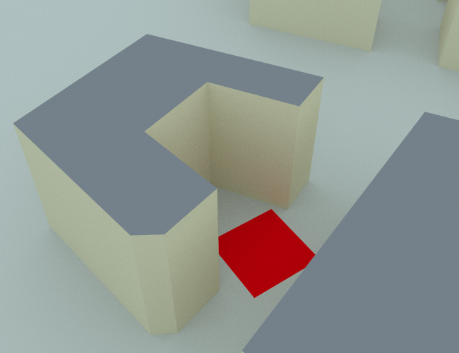
• Reconstruction performance evaluated on 210k independent locations within the red plane

\(100+\)x reduction in memory without major reconstruction error

RESULTS: MB-ML TRAINING DYNAMICS

• The MB-ML network quickly learns the correct scene (5 epochs represented here)

B. Chatelier, L. Le Magoarou, V. Corlay, M. Crussière, “Model-Based Learning for Multi-Antenna Multi-Frequency Location-to-Channel Mapping”, in IEEE JSTSP, 2024

APPLICATION TO RADIO-LOCALIZATION

• Given \(\bH\left(\bx\right)\), how to estimate \(\bx\)?

Problem 3.2: MB-ML for wireless localization

\[ \mini{\ftheta}{\espo{\norm{\textcolor{#B22222}{\ftheta\left(\bH\left(\bx\right)\right)}-\bx}{2}^2}{\left(\bx, \bH \left(\bx\right)\right) \sim p_{\bH,\bx}}}{\ftheta \in \mathcal{H}} \]

where:

\[ \begin{aligned} \textcolor{#B22222}{\ftheta} \colon \mbbC^{N_a \times N_s} &\longrightarrow \mbbR^3\\ \bH\left(\bx\right) &\longrightarrow \hat{\bx} \end{aligned} \]

• Goal: find \(\textcolor{#B22222}{\ftheta}\)
• Error measure: localization error (\(\ell_2\) norm)

• Fingerprinting-based localization:

\[ \hat{\bx}\left(\bH\left(\bx\right)\right) = \argmax{\tilde{\bx} \in \mathcal{G}} \simil{\bH\left(\bx\right),\bH\left(\tilde{\bx}\right)} \]

Drawback:

• Localization accuracy is limited by the dictionary resolution

B. Chatelier, V. Corlay, M. Furkan Keskin, M. Crussière, H. Wymeersch, L. Le Magoarou “Model-based Implicit Neural Representation for sub-wavelength Radio Localization”, submitted to IEEE TWC

Idea:

• Use the trained neural model to generate channel coefficients at wanted locations
  \(\rightarrow\) enhancing localization accuracy

• Use a physical channel model to guide an optimization process
  \(\rightarrow\) reducing complexity + improving performance

MB-ML paradigm application

Use the physical channel model to structure a neural architecture and optimize a gradient-descent process.

RESULTS

B. Chatelier, V. Corlay, M. Furkan Keskin, M. Crussière, H. Wymeersch, L. Le Magoarou “Model-based Implicit Neural Representation for sub-wavelength Radio Localization”, submitted to IEEE TWC

• Localization performance evaluated on 10k independent locations within the red plane

• Sub-wavelength localization accuracy

• \(10^{-1}\) cm \(\simeq 10^{-2} \lambda_0\)

\(100\)-\(1000\)x performance for \(10\)x less memory

KEY TAKEAWAYS

• Traditional MLPs suffer from the spectral bias and can not learn the location-to-channel mapping
• Using a physical channel model allows to structure a model-based neural network that overcomes this issue
• This network can be used to:
  • Perform channel reconstruction
  • Perform radio environment compression
  • Obtain sub-wavelength radio-localization performance

RESEARCH AXIS 2 Hardware impairments learning

Chapters 6 and 7 of the manuscript

MEASUREMENTS STRUCTURE

• In many communication problems, the measured signals \(\simeq\) noisy linear measurements of the channel \(\bh\):

  • parameterized by channel parameters (DoAs, delays…)
  • modeled as a linear combination of atomic channels (steering vectors, frequency response vectors…)
  • impacted by system parameters (antenna parameters, clock parameters…)

• Recover all the channel parameters (channel estimation/denoising)
  \(\rightarrow\) \(\bPsi_{\bzeta}\left(\bphi\right) \bs\)

• Recover part of the channel parameters (DoA/delay/gains estimation)
  \(\rightarrow\) \(\bphi\), \(\bs\)

• In actual systems, HWIs impact the system response

\(\bzeta^{\star}\) unknown \(\Rightarrow\bPsi_{\bzeta^{\star}} \left(\bphi\right)\) unknown

\(\bzeta\): system parameters

How to learn the true system parameters \(\bzeta^{\star}\)?

DoA : Direction of Arrival

HWIs : Hardware impairments

CHANNEL ESTIMATION (SISO-OFDM)

• Received signal: noisy linear combination of frequency response vectors
  • channel parameters: propagation delays \(\rightarrow \textcolor{#4682B4}{\bphi = \btau}\)

\[ \begin{align} \by &= \bh + \bn\\ & = \sum_{l=1}^{L_p} \alpha_l \bpsi_{\bzeta} \left(\tau_l\right) + \bn \end{align} \]

Problem 3.3.1: MB-ML for channel estimation

\[ \mini{\ftheta}{\espo{\norm{\textcolor{#B22222}{\ftheta\left(\by\right)}-\bh}{2}^2}{\left(\by, \bh \right) \sim p_{\by,\bh}}}{\ftheta \in \mathcal{H}} \]

where:

\[ \begin{aligned} \textcolor{#B22222}{\ftheta} \colon \mbbC^{N_s} &\longrightarrow \mbbC^{N_s}\\ \by &\longrightarrow \hat{\bh} \end{aligned} \]

• Goal: find \(\textcolor{#B22222}{\ftheta}\)
• Error measure: channel estimation error (\(\ell_2\) norm)

• Sparse recovery allows precise estimation if system parameters \(\bzeta\) are perfectly known:

\[ \text{Dictionary}: \bPsi_{\bzeta} = \left( \bpsi_{\bzeta}\left(\tau_1\right), \cdots, \bpsi_{\bzeta}\left(\tau_A\right) \right) \]

• Solve:

\[ \mini{\bu}{\norm{\bPsi_{\bzeta}\bu - \by }{2}}{\norm{\bu}{0}\leq A} \]

• Uncertain system parameters \(\Rightarrow\) Imperfect dictionary \(\Rightarrow\) Sub-optimal performance

• System parameters: gains, clock parameters

MB-ML paradigm application

Use the physical channel model to structure and initialize a neural network that learns HWIs.

MB-ML APPROACH: mpNet

• Unfolded version of the Matching Pursuit sparse recovery algorithm
  • Dictionary of frequency response vectors (variants for MIMO, MIMO-OFDM systems)

• Initialization: same behavior as the classical MP algorithm

• Training: learn system parameters \(\bzeta\) \(\rightarrow\) \(\abs{\bzeta}\) small (\(2N_s+1 = 513\) here)

• Optimization: avoid the full correlation \(\bPsi_{\bzeta}^\herm \by\) using a divide-and-conquer approach

T. Yassine and L. Le Magoarou, “mpNet: Variable Depth Unfolded Neural Network for Massive MIMO Channel Estimation”, in IEEE TWC, 2O22

B. Chatelier, L. Le Magoarou and G. Redieteab, “Efficient Deep Unfolding for SISO-OFDM Channel Estimation”, in IEEE ICC, 2023

N. Klaimi, A. Bedoui, C. Elvira, P. Mary and L. Le Magoarou, “Model-based learning for joint channel estimation and hybrid MIMO precoding”, in IEEE SPAWC, 2025

\(N_s\): number of frequencies

RESULTS

B. Chatelier, L. Le Magoarou and G. Redieteab, “Efficient Deep Unfolding for SISO-OFDM Channel Estimation”, in IEEE ICC, 2023

• Convergence to the perfect MB performance (known system parameters), in \(400\) channels

\(1000\)x reduction of learnable params., \(100\)x reduction of inference time

DOA ESTIMATION

D. H. Shmuel, J. P. Merkofer, G. Revach, R. J. G. van Sloun, N. Shlezinger “SubspaceNet: Deep Learning-Aided Subspace Methods for DoA Estimation” in IEEE TVT, 2025

DoA: Direction of Arrival

• Received signal: noisy linear combination of steering vectors
  • channel parameters: DoAs

\[ \bY = \bA_{\bzeta}\left(\bphi\right) \bS + \bN \]

• System parameters: antenna locations/gains

Problem 3.3.2: MB-ML for DoA estimation

\[ \mini{\ftheta}{\espo{\mu\left(\textcolor{#B22222}{\ftheta\left(\bY\right)},\bphi\right)}{\left(\bY, \bphi \right) \sim p_{\bY,\bphi}}}{\ftheta \in \mathcal{H}} \]

where:

\[ \begin{aligned} \textcolor{#B22222}{\ftheta} \colon \mbbC^{N_a \times T} &\longrightarrow \left[-\pi/2, \pi/2\right]^{M}\\ \bY &\longrightarrow \hat{\bphi} \end{aligned} \]

• Goal: find \(\textcolor{#B22222}{\ftheta}\)
• Error measure: angular estimation error (\(\mu \rightarrow\) RMSPE)

• MB approach: use of subspace methods \(\rightarrow\) MUltiple SIgnal Classification (MUSIC)

MUSIC: ILLUSTRATION

• MUSIC spectrum peaks at DoAs

DoA: Direction of Arrival

• MUSIC spectrum peaks at DoAs

What happens when the system parameters \(\bzeta\) are not perfectly known?

• Attenuated and offsetted MUSIC spectrum peaks with inaccurate \(\bzeta\)

MB-ML paradigm application

Use the physical channel model to structure and initialize a learning method for the HWIs.

MB-ML APPROACH: diffMUSIC

B. Chatelier, J. M. Mateos-Ramos, V. Corlay, C. Häger, M. Crussière, H. Wymeersch, L. Le Magoarou, “Physically Parameterized Differentiable MUSIC for DoA Estimation with Uncalibrated Arrays”, in IEEE ICC, 2025

A. Gast, L. Le Magoarou, N. Shlezinger “Near Field Localization via AI-Aided Subspace Methods”, 2025

\(N_a\): number of antennas

Idea:

Leverage gradient descent to solve:

\[ \mini{\bzeta}{\espo{\mu\left(\hat{\bphi}\left(\bY \vert \bzeta\right),\bphi\right)}{\left(\bY, \bphi \right) \sim p_{\bY,\bphi}}}{\bzeta \in \mathcal{H}_{\bzeta}} \]

Problem:

The peak-finding method breaks gradient flow \(\rightarrow\) MUSIC is non-differentiable wrt. \(\bzeta\)

How to overcome this issue?

• Initialization: Limited by the inaccurate \(\bzeta\)

• Training: Learn system parameters \(\bzeta\) \(\rightarrow\) \(\abs{\bzeta}\) small (\(3 N_a = 48\) here)

• Optimization: Task-specific supervised loss function, with theoretical performance guarantees

RESULTS

B. Chatelier, J. M. Mateos-Ramos, V. Corlay, C. Häger, M. Crussière, H. Wymeersch, L. Le Magoarou, “Physically Parameterized Differentiable MUSIC for DoA Estimation with Uncalibrated Arrays”, in IEEE ICC, 2025

• The MB-ML network reaches the perfect MB performance (known system parameters)

\(60\%\) reduction in estimation error for \(5\) sources

RESULTS: MB-ML TRAINING DYNAMICS

B. Chatelier, J. M. Mateos-Ramos, V. Corlay, C. Häger, M. Crussière, H. Wymeersch, L. Le Magoarou, “Physically Parameterized Differentiable MUSIC for DoA Estimation with Uncalibrated Arrays”, in IEEE ICC, 2025

• Learned \(\bzeta\) converges to true system parameters

• Peaks of the learned spectrum at the correct locations

KEY TAKEAWAYS

• HWIs impact the performance of many model-based methods
• MB-ML can be leveraged to structure and initialize learning methods for the system parameters impacted by HWIs
• This approach was used to:
  • Learn antenna gains and clock offsets in channel denoising
  • Learn antenna gains and locations in DoA estimation

HWIs: Hardware impairments

DoA: Direction of Arrival

RESEARCH AXIS 3 Efficient channel compression

Chapters 8 and 9 of the manuscript

CSI COMPRESSION IN FDD SYSTEMS

T. Yassine, B. Chatelier, V. Corlay, M. Crussière, S. Paquelet, O. Tirkkonen, L. Le Magoarou, “Model-Based Deep Learning for Beam Prediction Based on a Channel Chart” in IEEE ASILOMAR, 2023

B. Chatelier, V. Corlay, M. Crussière, L. Le Magoarou, “CSI Compresion using Channel Charting” in IEEE ASILOMAR, 2024

CSI: Channel State Information

FDD: Frequency Division Duplex

• Classical beamforming methods rely on the full CSI knowledge \(\rightarrow\) challenging in FDD systems

• Idea: encode the CSI at the UE side and decode it at the BS side

• High \(N_a N_s\) in modern systems \(\rightarrow\) costly reporting procedure

Problem 3.4: MB-ML for task-oriented CSI compression

\[ \mini{f_{\btheta_{\textsf{e}}}, \text{ } g_{\btheta_{\textsf{d}}}}{\espo{ \mu\left(\left(\textcolor{#4682B4}{g_{\btheta_\textsf{d}}} \circ \textcolor{#B22222}{f_{\btheta_\textsf{e}}}\right) \left(\bh\right), \bH \right) }{\bH \sim p_{\bH}}}{\left(f_{\btheta_\textsf{e}},g_{\btheta_\textsf{d}}\right) \in \mathcal{H}} \]

where: \[ \begin{aligned} \textcolor{#B22222}{f_{\btheta_\textsf{e}}} \colon \mbbC^{D} &\longrightarrow \mbbR^d\\ \bh &\longrightarrow \bz \end{aligned} \]

and:

\[ \begin{aligned} \textcolor{#4682B4}{g_{\btheta_\textsf{d}}} \colon \mbbR^d \times \cdots \times \mbbR^d &\longrightarrow \mbbC^{D\times K}\\ \left\{ \bz_1, \cdots, \bz_K \right\} &\longrightarrow \bW \end{aligned} \]

• Goal: find \(\textcolor{#B22222}{f_{\btheta_\textsf{e}}}\), \(\textcolor{#4682B4}{g_{\btheta_\textsf{d}}}\)
• Error measure: beamforming-based \(\rightarrow \mu\)

ENCODING: CHANNEL CHARTING

P. Ferrand, M. Guillaud, C. Studer and O. Tirkkonen, “Wireless Channel Charting: Theory, Practice, and Applications”, in IEEE Commun. Mag., 2023

• How to encode channels?

Channel charting: dimensionality reduction method that preserves local neighborhoods

• Channel \(\bh_i \in \mbbC^D\)

• Pseudo-loc. \(\bz_i = \textsf{E}\left(\bh_i\right) \in \mbbR^d\)
  \(\rightarrow\) \(d = 2\ll D = 1024\)

• Channel charting objective: \[ \norm{\bx_i - \bx_j}{2} \simeq \gamma \norm{\bz_i - \bz_j}{2} \]

MB-ML paradigm application

Use the physical channel model to structure and initialize a neural encoder/decoder.

MB-ML APPROACH

• A branch of channel charting is distance-based (ISOMAP)

• Idea: use a physical channel model to design a distance adapted to channel charting [Le Magoarou]

L. Le Magoarou, “Efficient channel charting via phase-insensitive distance computation”, in IEEE Wir. Commun. Lett., 2021

L. Le Magoarou, T. Yassine, S. Paquelet, and M. Crussière, “Channel charting based beamforming”, in IEEE ASILOMAR, 2022

T. Yassine, L. Le Magoarou, S. Paquelet, and M. Crussière, “Leveraging triplet loss and nonlinear dimensionality reduction for on-the-fly channel charting”, in IEEE SPAWC, 2022

OVERALL STRUCTURE

• Initialization: Using the ISOMAP algorithm

• Training: Task-specific loss function (known performance upon convergence)

• Optimization: Similarity-based subsampling [Taner et al.] \(\rightarrow\) reduce the number of learnable parameters

B. Chatelier, V. Corlay, M. Crussière, L. Le Magoarou, “CSI Compresion using Channel Charting” in IEEE ASILOMAR, 2024

S. Taner, M. Guillaud, O. Tirkkonen, C. Studer, “Channel charting for streaming CSI data”” in IEEE ASILOMAR, 2023

RESULTS

B. Chatelier, V. Corlay, M. Crussière, L. Le Magoarou, “CSI Compresion using Channel Charting” in IEEE ASILOMAR, 2024

• Improved beam alignment over the scene

• Good performance with high compression ratios, inter-UE interference cancellation

\(80\)x reduction of learnable params., \(16\)x increase in compression ratio

KEY TAKEAWAYS

• In FDD system, CSI feedback entails significant complexity
• MB-ML was leveraged to structure and initialize a neural encoder and decoder
• This allowed to:
  • Perform efficient CSI compression
  • Obtain good beamforming performance at high compression ratios
  • Obtain inter-UE interference cancellation without considering it during training

FDD: Frequency Division Duplex

CSI: Channel State Information

Conclusions and perspectives

CONCLUDING REMARKS

We have applied the MB-ML paradigm to several problems in wireless communications

• For learning the location-to-channel mapping
  • MB-ML allowed to structure a neural architecture
  • Excellent reconstruction performance and allows radio-environment compression

• For radio-localization
  • MB-ML allowed to structure a neural architecture and optimize a gradient-descent procedure
  • Sub-wavelength localization performance

• For HWIs compensation
  • MB-ML allowed to structure and initialize a neural architecture
  • Efficient joint HWIs compensation and parametric estimation

HWIs: Hardware Impairments

• For CSI compression
  • MB-ML allowed to structure and initialize a neural encoder/decoder
  • Improved compression ratios and good beamforming performance

CSI: Channel State Information

General advantages of MB-ML

• Increased interpretability

• Reduced complexity

• Well-suited for wireless communications

PERSPECTIVES

• Short term

  • Evaluate the proposed methods on real data
  • Investigate the location-to-channel mapping learning in an online learning setting with noisy channels
  • Leverage spatial augmentation techniques to get rid of the non-coherence assumption in diffMUSIC

• Long term

  • Leverage the location-to-channel model to perform imaging in the radio-environment
  • Evaluate the impact of the MB-ML structuration approach on the model’s neural tangent kernel

PUBLICATIONS

Journal articles

• Accepted: 1 (JSTSP)
• Under review: 1 (TWC)
• Planned: 1

International conference articles

• Accepted: 8 (ICC, ICASSP, ASILOMAR, ICMLCN, EuCNC, WCNC)

National conference articles

• Accepted: 1 (GRETSI)

Thanks!

Appendix

REFERENCES

• G. Peyré, “Manifold models for signals and images”, in Computer Vision and Image Understanding, 2009
• M. Elad, “Sparse and Redundant Representations: From Theory to Applications in Signal and Image Processing”, Springer, 2010
• Nir Shlezinger, Yonina C. Eldar, “Model-Based Deep Learning”, Foundations and Trends in Signal Processing, 2023
• J. Hoydis et al., “Sionna: An Open-Source Library for Next-Generation Physical Layer Research”, 2022
• K. Hornik, M. Stinchcombe, and H. White, “Multilayer feedforward networks are universal approximators”, in Neural Networks, 1989
• G. Cybenko, “Approximation by superpositions of a sigmoidal function”, in Mathematics of Controls, Signals and Systems, 1989
• N. Rahaman et al., “On the spectral bias of neural networks”, in ICML, 2019
• Y. Cao et al., “Towards Understanding the Spectral Bias of Deep Learning”, in IJCAI, 2021
• B. Chatelier, L. Le Magoarou, V. Corlay, M. Crussière, “Model-Based Learning for Location-to-Channel Mapping”, in IEEE ICASSP, 2024
• B. Chatelier, L. Le Magoarou, V. Corlay, M. Crussière, “Model-Based Learning for Multi-Antenna Multi-Frequency Location-to-Channel Mapping”, in IEEE JSTSP, 2024

REFERENCES

• B. Chatelier, V. Corlay, M. Furkan Keskin, M. Crussière, H. Wymeersch, L. Le Magoarou “Model-based Implicit Neural Representation for sub-wavelength Radio Localization”, submitted to IEEE TWC
• T. Yassine and L. Le Magoarou, “mpNet: Variable Depth Unfolded Neural Network for Massive MIMO Channel Estimation”, in IEEE TWC, 2O22
• B. Chatelier, L. Le Magoarou and G. Redieteab, “Efficient Deep Unfolding for SISO-OFDM Channel Estimation”, in IEEE ICC, 2023
• N. Klaimi, A. Bedoui, C. Elvira, P. Mary and L. Le Magoarou, “Model-based learning for joint channel estimation and hybrid MIMO precoding”, in IEEE SPAWC, 2025
• D. H. Shmuel, J. P. Merkofer, G. Revach, R. J. G. van Sloun, N. Shlezinger “SubspaceNet: Deep Learning-Aided Subspace Methods for DoA Estimation” in IEEE TVT, 2025
• B. Chatelier, J. M. Mateos-Ramos, V. Corlay, C. Häger, M. Crussière, H. Wymeersch, L. Le Magoarou, “Physically Parameterized Differentiable MUSIC for DoA Estimation with Uncalibrated Arrays”, in IEEE ICC, 2025
• B. Chatelier, V. Corlay, M. Crussière, L. Le Magoarou, “CSI Compresion using Channel Charting” in IEEE ASILOMAR, 2024
• T. Yassine, B. Chatelier, V. Corlay, M. Crussière, S. Paquelet, O. Tirkkonen, L. Le Magoarou, “Model-Based Deep Learning for Beam Prediction Based on a Channel Chart” in IEEE ASILOMAR, 2023

REFERENCES

• P. Ferrand, M. Guillaud, C. Studer and O. Tirkkonen, “Wireless Channel Charting: Theory, Practice, and Applications”, in IEEE Commun. Mag., 2023
• L. Le Magoarou, “Efficient channel charting via phase-insensitive distance computation”, in IEEE Wir. Commun. Lett., 2021
• L. Le Magoarou, T. Yassine, S. Paquelet, and M. Crussière, “Channel charting based beamforming”, in IEEE ASILOMAR, 2022
• T. Yassine, L. Le Magoarou, S. Paquelet, and M. Crussière, “Leveraging triplet loss and nonlinear dimensionality reduction for on-the-fly channel charting”, in IEEE SPAWC, 2022
• S. Taner, M. Guillaud, O. Tirkkonen, C. Studer, “Channel charting for streaming CSI data”” in IEEE ASILOMAR, 2023

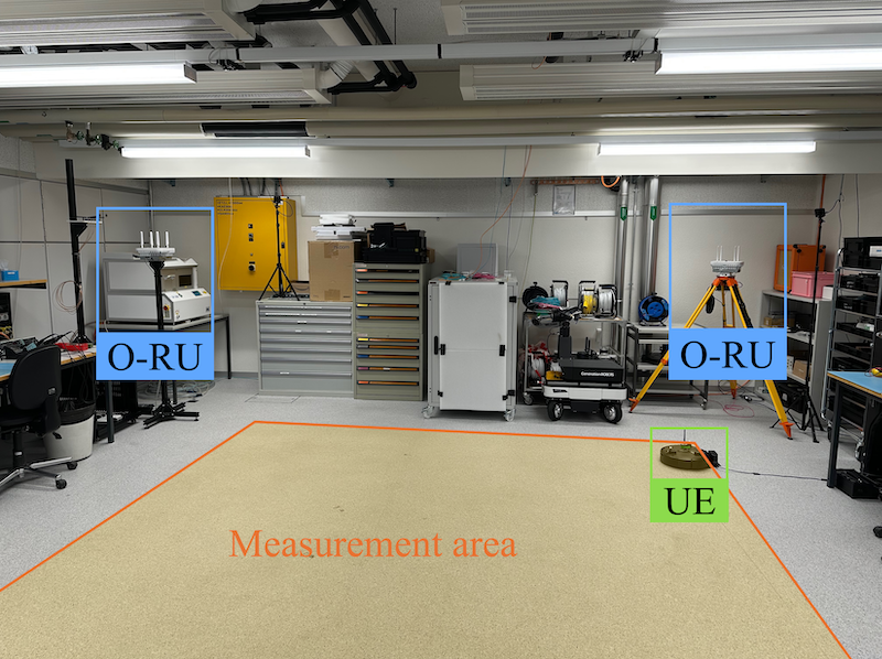
REAL CHANNEL DATASETS

• For channel charting: DICHASUS

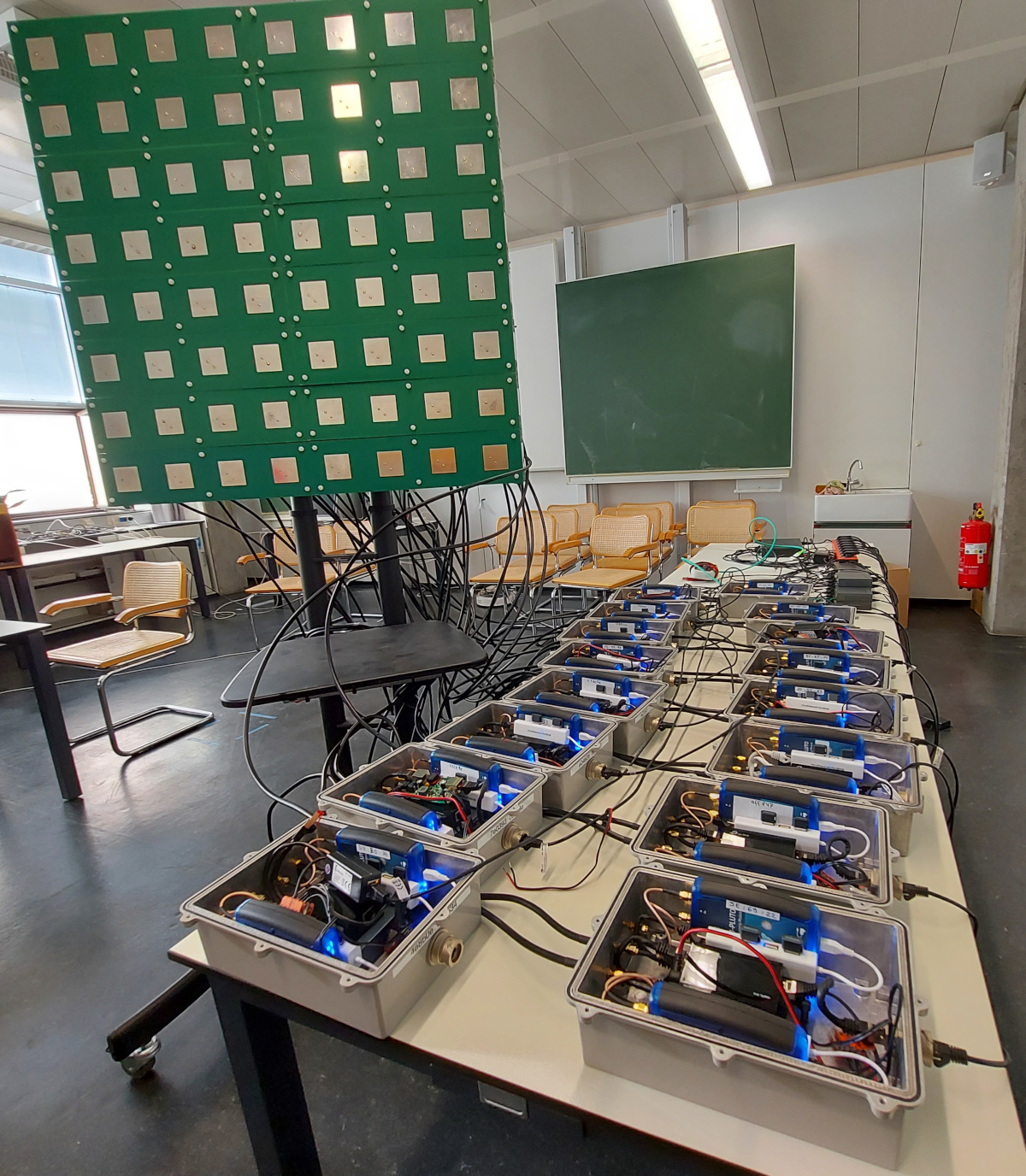
• For the location-to-channel mapping: CAEZ-5G/WiFi

F. Euchner, M. Gauger, S. Doerner, S. ten Brink, “A Distributed Massive MIMO Channel Sounder for “Big CSI Data”-driven Machine Learning”, in IEEE WSA, 2021

R. Wiesmayr, F. Zumegen, S. Taner, C. Dick, C. Studer, “CSI-Based User Positioning, Channel Charting, and Device Classification with an NVIDIA 5G Testbed”, in IEEE ASILOMAR, 2025

MODEL-BASED MACHINE LEARNING: USE CASES

• MB-ML is relevant when both MB methods and ML methods exhibits shortcomings

• MB inaccurate and ML too slow/too complex to train
  \(\rightarrow\) too many parameters/requires too much data

• MB too complex/ML not approriate
  \(\rightarrow\) no obvious approach

Use case examples:

Resilient parametric estimation, dynamic system tracking, channel decoding, ISAC system design…

CHANNEL MODEL

Assumption: attenuation/phase proportional to the propagation distance

\[ \begin{align} h_{j,k}\left(\mathbf{x}\right) &= \sum_{l=1}^{L_p} \dfrac{\alpha_l \mathrm{e}^{\mathrm{j}\beta_l}}{d_l\left(\mathbf{x}\right)} \mathrm{e}^{-\mathrm{j}\frac{2\pi}{\lambda_k}d_l\left(\mathbf{x}\right)}\\ &\hphantom{\sum_{l=1}^{L_p} \dfrac{\alpha_l \mathrm{e}^{\mathrm{j}\beta_l}}{\norm{\mathbf{x}-\mathbf{a}_{l,j}}{2}} \mathrm{e}^{-\mathrm{j}\frac{2\pi}{\lambda_k}\norm{\mathbf{x}-\mathbf{a}_{l,j}}{2}}} \notag % &= \sum_{l=1}^{L_p} \dfrac{\alpha_l \mathrm{e}^{\mathrm{j}\beta_l}}{\norm{\mathbf{x}-\mathbf{a}_{l,j}}{2}} \mathrm{e}^{-\mathrm{j}\frac{2\pi}{\lambda_k}\norm{\mathbf{x}-\mathbf{a}_{l,j}}{2}} \end{align} \]

\[ \begin{align} h_{j,k}\left(\mathbf{x}\right) &= \sum_{l=1}^{L_p} \dfrac{\alpha_l \mathrm{e}^{\mathrm{j}\beta_l}}{d_l\left(\mathbf{x}\right)} \mathrm{e}^{-\mathrm{j}\frac{2\pi}{\lambda_k}d_l\left(\mathbf{x}\right)} \tag{22}\\ &= \sum_{l=1}^{L_p} \dfrac{\alpha_l \mathrm{e}^{\mathrm{j}\beta_l}}{\norm{\mathbf{x}-\mathbf{a}_{l,j}}{2}} \mathrm{e}^{-\mathrm{j}\frac{2\pi}{\lambda_k}\norm{\mathbf{x}-\mathbf{a}_{l,j}}{2}} \end{align} \]

\[ \begin{align} h_{j,k}\left(\mathbf{x}\right) &= \sum_{l=1}^{L_p} \dfrac{\alpha_l \mathrm{e}^{\mathrm{j}\beta_l}}{d_l\left(\mathbf{x}\right)} \mathrm{e}^{-\mathrm{j}\frac{2\pi}{\lambda_k}d_l\left(\mathbf{x}\right)} \tag{22}\\ &= \sum_{l=1}^{L_p} \dfrac{\alpha_l \mathrm{e}^{\mathrm{j}\beta_l}}{\norm{\mathbf{x}-\mathbf{a}_{l,j}}{2}} \mathrm{e}^{-\mathrm{j}\frac{2\pi}{\lambda_k}\norm{\mathbf{x}-\mathbf{a}_{l,j}}{2}} \tag{23}\\ &= \sum_{l=1}^{L_p} \dfrac{\alpha_l \mathrm{e}^{\mathrm{j}\beta_l}}{d_l\left(\mathbf{x}\right)} \mathrm{e}^{-\mathrm{j} 2\pi f_k \tau_{l,j} } \end{align} \]

TAYLOR EXPANSIONS

\[ \norm{\mathbf{x}-\mathbf{a}_{l,j}}{2} \simeq \textcolor{black}{\norm{\mathbf{x}_r - \mathbf{a}_{l,r}}{2}} \textcolor{black}{+ \mathbf{u}_{l,j}\left(\mathbf{x}_r\right)^\transp\left(\mathbf{x}-\mathbf{x}_r\right)} \textcolor{black}{- \mathbf{u}_{l,r}\left(\mathbf{x}_r\right)^\transp \left(\mathbf{a}_{l,j}-\mathbf{a}_{l,r}\right)} \]

\[ \textcolor{#FF1B17}{\norm{\mathbf{x}-\mathbf{a}_{l,j}}{2}} \simeq \textcolor{black}{\norm{\mathbf{x}_r - \mathbf{a}_{l,r}}{2}} \textcolor{black}{+ \mathbf{u}_{l,j}\left(\mathbf{x}_r\right)^\transp\left(\mathbf{x}-\mathbf{x}_r\right)} \textcolor{black}{- \mathbf{u}_{l,r}\left(\mathbf{x}_r\right)^\transp \left(\mathbf{a}_{l,j}-\mathbf{a}_{l,r}\right)} \tag{25} \]

\[ \textcolor{#FF1B17}{\norm{\mathbf{x}-\mathbf{a}_{l,j}}{2}} \simeq \textcolor{#0D00BA}{\norm{\mathbf{x}_r - \mathbf{a}_{l,r}}{2}} \textcolor{black}{+ \mathbf{u}_{l,j}\left(\mathbf{x}_r\right)^\transp\left(\mathbf{x}-\mathbf{x}_r\right)} \textcolor{black}{- \mathbf{u}_{l,r}\left(\mathbf{x}_r\right)^\transp \left(\mathbf{a}_{l,j}-\mathbf{a}_{l,r}\right)} \tag{25} \]

\[ \textcolor{#FF1B17}{\norm{\mathbf{x}-\mathbf{a}_{l,j}}{2}} \simeq \textcolor{#0D00BA}{\norm{\mathbf{x}_r - \mathbf{a}_{l,r}}{2}} \textcolor{#62BE00}{+ \mathbf{u}_{l,j}\left(\mathbf{x}_r\right)^\transp\left(\mathbf{x}-\mathbf{x}_r\right)} \textcolor{black}{- \mathbf{u}_{l,r}\left(\mathbf{x}_r\right)^\transp \left(\mathbf{a}_{l,j}-\mathbf{a}_{l,r}\right)} \tag{25} \]

\[ \textcolor{#FF1B17}{\norm{\mathbf{x}-\mathbf{a}_{l,j}}{2}} \simeq \textcolor{#0D00BA}{\norm{\mathbf{x}_r - \mathbf{a}_{l,r}}{2}} \textcolor{#62BE00}{+ \mathbf{u}_{l,j}\left(\mathbf{x}_r\right)^\transp\left(\mathbf{x}-\mathbf{x}_r\right)} \textcolor{#FF8A00}{-\mathbf{u}_{l,r}\left(\mathbf{x}_r\right)^\transp \left(\mathbf{a}_{l,j}-\mathbf{a}_{l,r}\right)} \tag{25} \]

\[ \textcolor{#FF1B17}{\norm{\mathbf{x}-\mathbf{a}_{l,j}}{2}} \simeq \textcolor{#0D00BA}{\norm{\mathbf{x}_r - \mathbf{a}_{l,r}}{2}} \textcolor{#62BE00}{+ \mathbf{u}_{l,j}\left(\mathbf{x}_r\right)^\transp\left(\mathbf{x}-\mathbf{x}_r\right)} \textcolor{#FF8A00}{-\mathbf{u}_{l,r}\left(\mathbf{x}_r\right)^\transp \left(\mathbf{a}_{l,j}-\mathbf{a}_{l,r}\right)} \tag{25} \]

\[ \textcolor{#FF1B17}{\norm{\mathbf{x}-\mathbf{a}_{l,j}}{2}} \simeq \textcolor{#0D00BA}{\norm{\mathbf{x}_r - \mathbf{a}_{l,r}}{2}} \textcolor{#62BE00}{+ \mathbf{u}_{l,j}\left(\mathbf{x}_r\right)^\transp\left(\mathbf{x}-\mathbf{x}_r\right)} \textcolor{#FF8A00}{-\mathbf{u}_{l,r}\left(\mathbf{x}_r\right)^\transp \left(\mathbf{a}_{l,j}-\mathbf{a}_{l,r}\right)} \tag{25} \]

\[ \textcolor{#FF1B17}{\norm{\mathbf{x}-\mathbf{a}_{l,j}}{2}} \simeq \textcolor{#0D00BA}{\norm{\mathbf{x}_r - \mathbf{a}_{l,r}}{2}} \textcolor{#62BE00}{+ \mathbf{u}_{l,j}\left(\mathbf{x}_r\right)^\transp\left(\mathbf{x}-\mathbf{x}_r\right)} \textcolor{#FF8A00}{-\mathbf{u}_{l,r}\left(\mathbf{x}_r\right)^\transp \left(\mathbf{a}_{l,j}-\mathbf{a}_{l,r}\right)} \tag{25} \]

\[ \textcolor{#FF1B17}{\norm{\mathbf{x}-\mathbf{a}_{l,j}}{2}} \simeq \textcolor{#0D00BA}{\norm{\mathbf{x}_r - \mathbf{a}_{l,r}}{2}} \textcolor{#62BE00}{+ \mathbf{u}_{l,j}\left(\mathbf{x}_r\right)^\transp\left(\mathbf{x}-\mathbf{x}_r\right)} \textcolor{#FF8A00}{-\mathbf{u}_{l,r}\left(\mathbf{x}_r\right)^\transp \left(\mathbf{a}_{l,j}-\mathbf{a}_{l,r}\right)} \tag{25} \]

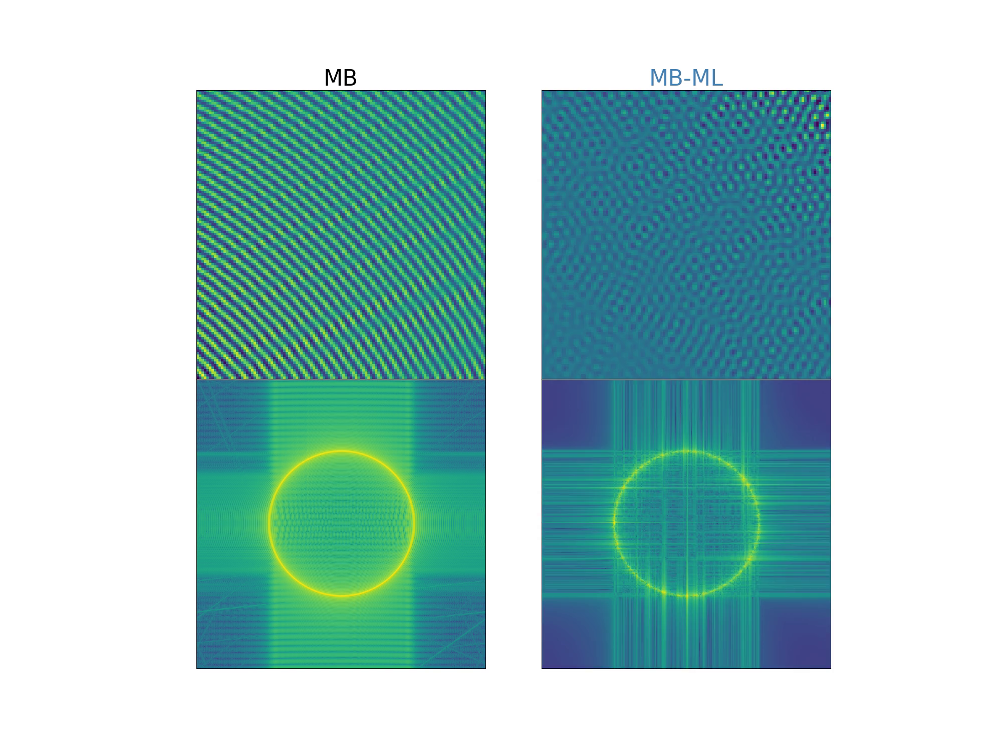
RECONSTRUCTION RESULTS

PROPOSED LOCALIZATION METHOD

• Based on grid-search and gradient descent, using a Frobenius norm similarity measure:

\[ \mu_{\textsf{PS}}\left(\bH\left(\bx\right), \tilde{\bx} \vert \btheta \right) = \norm{\bH\left(\bx\right) - \ftheta\left(\tilde{\bx}\right)}{\mathsf{F}} \]

Chatelier et al., “Model-based Implicit Neural Representation for sub-wavelength Radio Localization”.

• How to estimate \(\bx\)?
• Background: \(\norm{\bH\left(\bx\right) - \ftheta\left(\tilde{\bx}\right)}{\mathsf{F}}\)

• Generate the global grid \(\mathcal{G}_{\textsf{G}}\) based on topological knowledge of the scene

• Generate the global grid \(\mathcal{G}_{\textsf{G}}\) based on topological knowledge of the scene
• Using \(\ftheta\), solve:

\[ \tilde{\bx}_{\textrm{i}} = \argmin{\tilde{\bx} \in \mathcal{G}_{\textsf{G}}} \norm{\bH\left(\bx\right) - \ftheta\left(\tilde{\bx}\right)}{\mathsf{F}} \]

• Generate the local grid \(\mathcal{G}_{\textsf{L}}\) around the obtained location

• Generate the local grid \(\mathcal{G}_{\textsf{L}}\) around the obtained location
• Using \(\ftheta\), solve:

\[ \tilde{\bx}_{\textrm{g}} = \argmin{\tilde{\bx} \in \mathcal{G}_{\textsf{L}}} \norm{\bH\left(\bx\right) - \ftheta\left(\tilde{\bx}\right)}{\mathsf{F}} \]

• Perform \(N_{\nabla}\) gradient descent steps

• Perform \(N_{\nabla}\) gradient descent steps

• Perform \(N_{\nabla}\) gradient descent steps

• Perform \(N_{\nabla}\) gradient descent steps

• Perform \(N_{\nabla}\) gradient descent steps
• Local minima issue

• Perform \(N_{\nabla}\) gradient descent steps
• Local minima issue
• Spacing between minima derived from \(\mu_{\textsf{PS}}\)

• Perform \(N_{\nabla}\) gradient descent steps
• Local minima issue
• Spacing between minima derived from \(\mu_{\textsf{PS}}\)
• Generate circles of radius \(k\lambda_0, k \in \mbbN^*\)

• Perform \(N_{\nabla}\) gradient descent steps
• Local minima issue
• Spacing between minima derived from \(\mu_{\textsf{PS}}\)
• Generate circles of radius \(k\lambda_0, k \in \mbbN^*\)
• Generate \(\mathcal{G}_{\textsf{C}}\) by sampling for the circles

• Perform \(N_{\nabla}\) gradient descent steps
• Local minima issue
• Spacing between minima derived from \(\mu_{\textsf{PS}}\)
• Generate circles of radius \(k\lambda_0, k \in \mbbN^*\)
• Using \(\ftheta\), solve:

\[ \tilde{\bx}_{\textrm{c}^{\star}} = \argmin{\tilde{\bx} \in \mathcal{G}_{\textsf{C}}} \norm{\bH\left(\bx\right) - \ftheta\left(\tilde{\bx}\right)}{\mathsf{F}} \]

• Perform \(N_{\nabla}\) gradient descent steps

• Perform \(N_{\nabla}\) gradient descent steps

• Perform \(N_{\nabla}\) gradient descent steps

We used the MB-ML paradigm to structure a neural architecture and optimize a gradient-descent process

LOCALIZATION RESULTS

• Localization performance evaluated on 10k independent locations within the red planes

SNR=5dB

DIVIDE-AND-CONQUER

diffMUSIC PRINCIPLES

PI DISTANCE

Solution [Le Magoarou]: Phase-insensitive distance

\[ d\left(\bh_i, \bh_j\right) = \sqrt{2-2 \frac{\abs{\bh_i^\herm \bh_j}}{\norm{\bh_i}{2} \norm{\bh_j}{2}}} \]

CELL-FREE SYSTEM

MONO-UE PERFORMANCE (SUBSAMPLING)

• Subsampling does not impact mono-UE beamforming performance

LINKING CHANNEL CHARTING AND SOURCE CODING

B. Park, H. Do, N. Lee, “Transformer-Based Nonlinear Transform Coding for Multi-Rate CSI Compression in MIMO-OFDM Systems”, in IEEE ICC, 2025

SERMENT DOCTORAL

French version

En présence de mes pairs.

Parvenu à l’issue de mon doctorat en traitement du signal, et ayant ainsi pratiqué, dans ma quête du savoir, l’exercice d’une recherche scientifique exigeante, en cultivant la rigueur intellectuelle, la réflexivité éthique et dans le respect des principes de l’intégrité scientifique, je m’engage, pour ce qui dépendra de moi, dans la suite de ma carrière professionnelle, quel qu’en soit le secteur ou le domaine d’activité, à maintenir une conduite intègre dans mon rapport au savoir, mes méthodes et mes résultats.

English version

In the presence of my peers.

With the completion of my doctorate in signal processing, in my quest for knowledge, I have carried out demanding research, demonstrated intellectual rigour, ethical reflection, and respect for the principles of research integrity. As I pursue my professional career, whatever my chosen field, I pledge, to the greatest of my ability, to continue to maintain integrity in my relationship to knowledge, in my methods and in my results. ​